What are MMMs and what are they used for?
An important part of any business is marketing. By successfully allocating your marketing budget to the right marketing channels, you can increase your revenue or reduce your marketing costs while keeping the same revenue. But deciding how to allocate your marketing budget optimally is easier said than done. MMMs are exactly designed for this purpose. An MMM model will find how effective (or ineffective) different marketing channels are. Once you know this relationship you can optimize your marketing budget accordingly.
One of the leading approaches to MMM models is the open-source package Robyn, developed by Meta. Robyn makes it easy for anyone with a basic understanding of programming in R to set up a MMM model and run a budget optimization. You load in your marketing expenditures and your revenue and Robyn will do the rest. Due to its ease of use, Robyn is becoming the industry standard for MMM models. But unfortunately, Robyn has quite a few shortcomings and limitations you should consider.
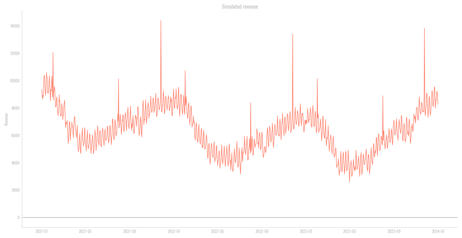
To demonstrate Robyn’s shortcomings and limitations, we decided to put it to the test using a simulated data set. With a simulated data set, we will be able to see how well Robyn will perform since we know the underlying mechanics behind this data set. We can, for example, configure how each of the marketing channels impacts revenue. This allows us to validate if the Robyn models found the same degree of importance.
Simulated Dataset
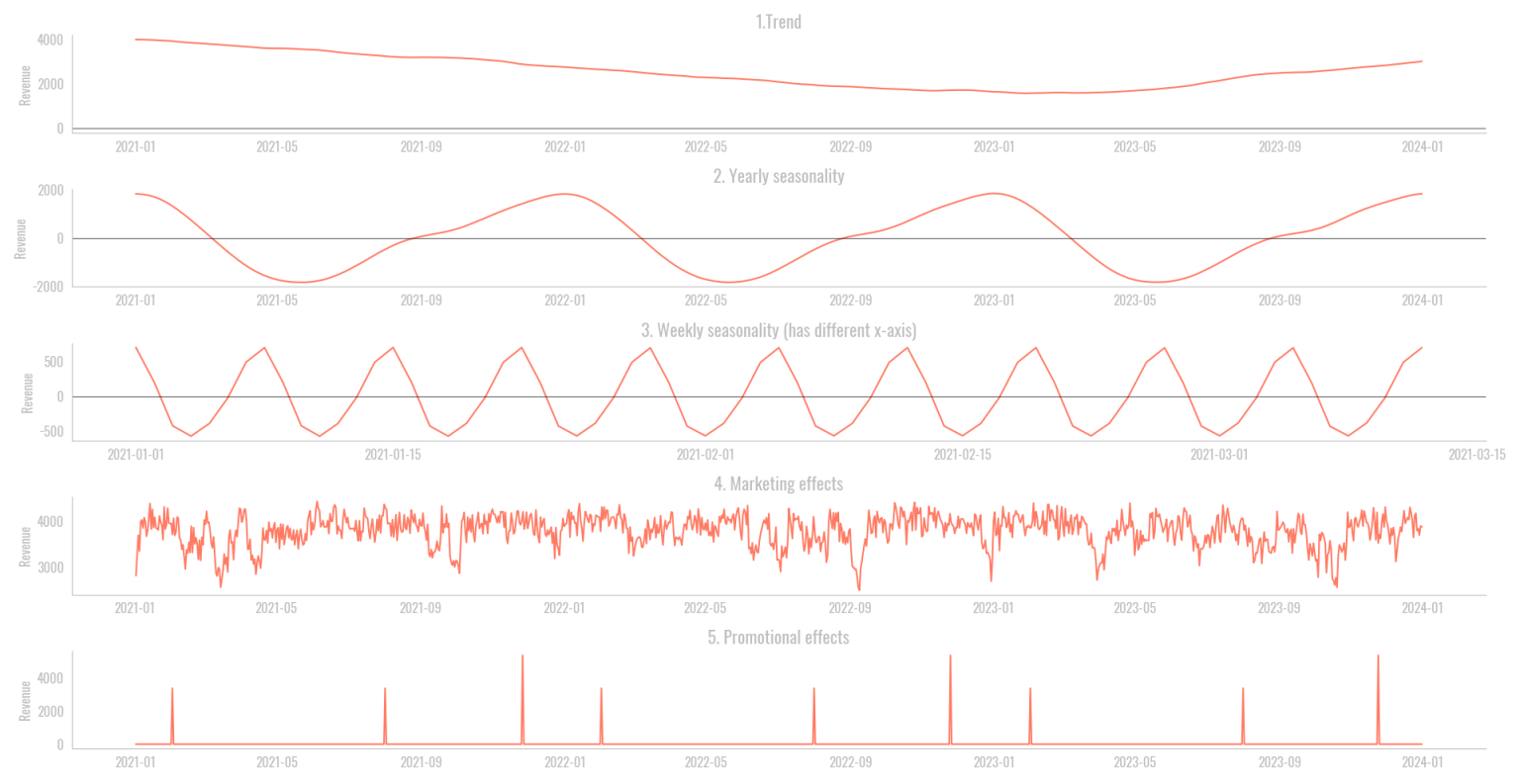
The simulated dataset we will be using consists of five different components that we expect to find in any real data set. Each of these five components contributes to the revenue. Using these five components we will simulate the revenue for three years. Below you can see a breakdown of the simulated dataset:
The first component is the general trend or your baseline sales. It’s generated independent of the time of the year or your marketing spending. The second component is the yearly season, which models the fact that in a specific part of the year, more revenue is generated than in other parts of the year. The third component is the weekly season, which is the same as the yearly season but on a weekly time scale. The fourth component is the one we are interested in: the effect your marketing spend has on revenue. We will be using 8 different marketing channels. Lastly, we also included 3 promotional events in the year where a lot of extra revenue is generated. An overview of each of the components can be seen below:
The relationship between ad spend & revenue
At the heart of an MMM lies its budget optimization capabilities, it lets you find the relation between your marketing spend and the revenue. However, this relation is not linear. As you spend more and more in one channel the returns of this channel will start to diminish; this is also known as channel saturation. This effect can be modeled using a saturation curve.
The main task Robyn carries out is to estimate these saturation curves. If you can correctly identify these curves you will also be able to find the optimal budget allocation which maximizes your revenue. If on the other hand, you fail to find the correct saturation curves you won’t be able to find the best budget allocation. And even worse, your new budget allocation can lead to a decrease in revenue. Exactly the opposite of what you want.
We let Robyn estimate the saturation curves for our 8 different marketing channels. It is important to note that Robyn does not come up with just one model when it tries to optimize your budget, instead, it finds anywhere between 2 and 14 “best” models. We selected the first 4 best models Robyn found while optimizing the simulated data set. The results can be seen in the figure below:
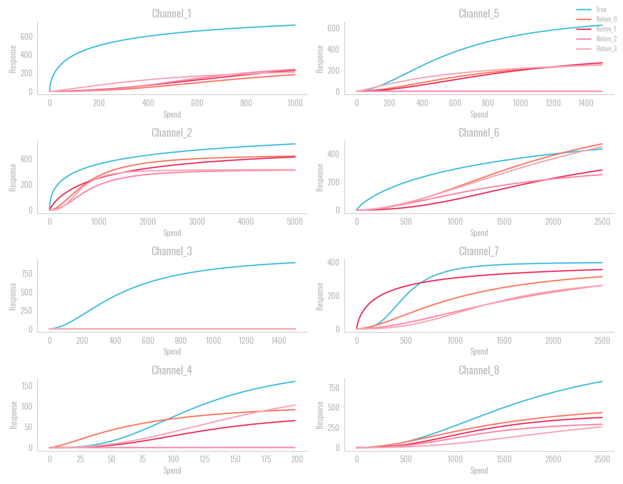
When looking at the figures, it can be seen that Robyn was not able to accurately estimate the true saturation curves for almost all the channels. Most of the time it greatly underestimates the influence each channel has on the revenue. This is most apparent in channel 3, where Robyn deemed the channel to be completely insignificant. But the exact opposite is the case since channel 3 has actually one of the strongest effects on the revenue (see the y-axis). These wrongly estimated saturation curves have a severe impact on the budget optimization.
Missed opportunity
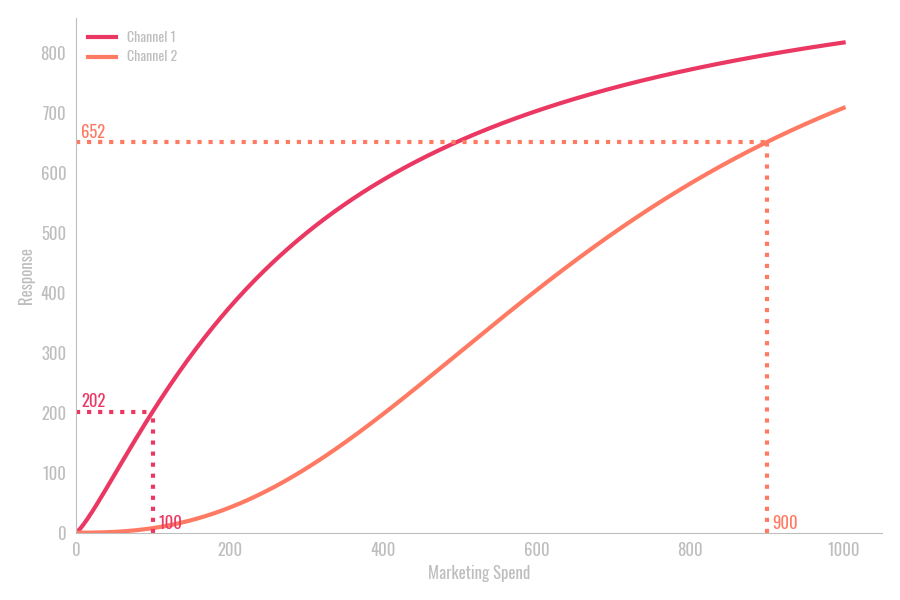
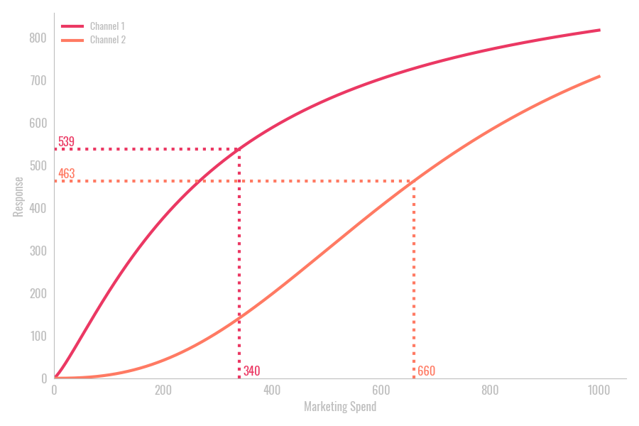
How exactly do these saturation curves translate into an optimal budget? Let us demonstrate this with a small example. Assume your total marketing budget is $1000 and you have two marketing channels to spend on. You spend a lot of this $1000 in Channel 1, say $900, and a little in the other, $100. Using the saturation curves of each channel we can see that this results in an expected revenue of $652 + $202 = $854 (see left plot below).
We used this same principle using the saturation curves Robyn found for each of our 8 marketing channels. Since Robyn performs poorly at finding the saturation curves, the budget allocation is unfortunately also quite bad. In 3 of the 4 models, following the budget reallocation of Robyn leads to a decrease in revenue compared to the original revenue of the simulated data set. The results can be seen in the table below:
Model | Before | After (Robyn) | Increase (Robyn) |
Robyn_0 | € 2,591,259.16 | € 2,673,925.98 | 3.19% |
Robyn_1 | € 2,591,259.16 | € 2,416,672.25 | -6.74% |
Robyn_2 | € 2,591,259.16 | € 2,471,183.28 | -4.63% |
Robyn_3 | € 2,591,259.16 | € 2,516,982.67 | -2.87% |
To make sure this is not just a fluke, we repeated the same process described above for 100 different datasets. For each of these datasets we let Robyn estimate the saturation curves and using these saturation curves we found an increase or decrease in the revenue. Since we also know the true saturation curves, we were also able to find the optimal possible revenue increase for each of the datasets. The results can be seen in the figure below:
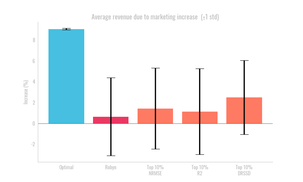
On average the potential revenue increase sits around 9% as can be seen when looking at the left bar of the figure. Robyn only found an average increase of 0.7%. But as mentioned earlier, it often actually led to a decrease in revenue. When processing the 100 datasets it found 758 best models. Of these 758 models 315 of them would lead to a decrease in revenue, around 42% of the time.
Since Robyn comes up with multiple best models per dataset, it is sometimes hard to determine which one to use. To solve this problem, we can look at the 3 different fit metrics Robyn uses to determine its best models. These are the NRMSE, R-squared (R2) and DRSSD. So, we also computed the average revenue increase of the top 10% models of the top 758 models for each of these three fit metrics. As can be seen in the figure, the total average revenue increase went up but is still not close to the optimal increase. And once again a lot of these top 10% models would also lead to a revenue decrease.
Conclusion
As demonstrated, optimally allocating your marketing budget can be challenging. Even large tech companies like Meta face difficulties in implementing robust solutions as their MMM approach often results in decreased revenue. Fortunately, there are alternatives to using Robyn. If you’re interested in exploring better solutions or discussing your approach to MMMs, feel free to get in touch.